Is There an Optimal Size for Magrid Casings?

[Betruger]

I'm sorry, slipped my mind. Here it is.

[tombo]

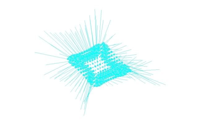
This porcupine is a snapshot of a work in progress so please don't be too harsh in your judgment.
It has been so long since I contributed that I wanted to get something showing.

I started with Kiteman's spreadsheet, tore my hair out trying to figure out how it works & rejiggered it to make it do what I wanted. [excel was obviously written by and for accountants not engineers. They just don't think the same way on some fundamental level. All of the things it can do seem to go at right angles to what I want to do.]

What you see here is the B field on a plane like Kiteman's excel charts. The X-Cusp one.
This is a very coarse version to speed things up.
I made excel generate a script file to feed into AutoCAD to draw the field vectors on a grid.
I did another earlier to generate the wire path from the excel list of points you integrated along, but I did not post it because it is not visually interesting. And I need to get some sleep. Making the wire paths 3-D should be relatively straightforward.

This is (supposed to be) the magnetic field vectors. The ball is centered on the grid point, the ball diameter and the stick length are proportional to the field strength and the direction of the stick is the field direction.
The next step is to get it to show the field in more planes. Easy by hand except for writer's cramp. So I have to automate it somehow.
After that I want to get the free viewer off the AutoCAD website and find a way to link to that and post this so you all can turn it to any angle and zoom in and out to really see how the fields go. Supposedly the free Autodesk Design Review program will allow you to view, print, measure, mark up, and revise 2D and 3D designs with or without the original design-creation software.

This process should be a great help to all of us trying to show each other 3-D objects and fields etc.

If you want to see Kiteman's excel charts of the fields better, try downloading the excel file then right clicking in the chart area and choosing 3-D view.
It will let you look at them from different angles which is VERY enlightening.
.
Then I want to increase resolution to make it more meaningful

Once all that is up and running the real fun starts: trying it out on other coil configurations.

Also:
Kiteman,
Is there a reason for the yellow highlighted cells? There are 4 at -25 by 35.
I use that color as a warning but they seem harmless enough. Should I be worried?
I don't follow your logic between the summation of the fields and the output to the chart at S52.
I used Bx=P52, By=R52 & Bz=S52 OK?
What is the scale of the B values?

[KitemanSA]

I started with Kiteman's spreadsheet, tore my hair out trying to figure out how it works & rejiggered it to make it do what I wanted.

Welcome to my world.

Also:
Kiteman,
Is there a reason for the yellow highlighted cells? There are 4 at -25 by 35.
I use that color as a warning but they seem harmless enough. Should I be worried?

No you need not be worried. They were modeling markers that I neglected to erase.

I don't follow your logic between the summation of the fields and the output to the chart at S52.

I modeled two superposed half symmetric models, one for the side/side loops and one for the top/bottom loops. The summations at Q, R, and S; then again at Z, AA, & AB give the x, y, and z fields for the selected point in the upper left and lower right quarter fields respectively for each half-sym model. O51 superposes the “x” field of the modeled side coil with that of the “other” (unmodeled) side while O53 does the same for the modeled top and the unmodeled bottom. O52 is the superposition of the side/side with the top/bottom with a multiplier of 100 just to get the numbers into a reasonable range. Q52 and R52 do the same for the “y” and “z” fields respectively. S52 selects which field, tangential (root sum squares of x&y) or radial (z) to put into the table based on the value in F1 of that sheet.

I used Bx=P52, By=R52 & Bz=S52 OK?

Not sure what you mean here. There is no P52. O52, Q52, and R52 are the summed Bx, By, and Bz respectively.

What is the scale of the B values?

They have no scale. I used arbitrary units of distance and amp-turns and did not include any constants. These values are all relative to an arbitrary unit.

(deleted spurious "1" from "R521".)

[tombo]

O52, Q52, and R521 are the summed Bx, By, and Bz respectively.

Yes that is what I meant.
These are where I am taking your output as my input to run with.

O51 superposes the “x” field of the modeled side coil with that of the “other” (unmodeled) side while O53 does the same for the modeled top and the unmodeled bottom. O52 is the superposition of the side/side with the top/bottom with a multiplier of 100 just to get the numbers into a reasonable range.

By unmodeled do you mean not shown in columns A, B & C?
They look modeled to me when I look at columns Z, AA & AB.
(I think this is just semantics.)
I will want to make these 4 wire segments explicit and independent before I can apply this model to the further problems that I have in mind.
I think that will be easy enough. Do you concur?

I used arbitrary units of distance and amp-turns and did not include any constants. These values are all relative to an arbitrary unit.

That was what I was afraid of.

I think I can turn the units into T by multiplying by 10e-7 (=mu0/4*pi) instead of by 100 at cells O52, Q52 & R52.
Are the length units real units? Or, do I need to convert them to meters of an actual machine to be modeled too?
I suppose I have to because none of the models we are considering for the near term are anywhere near 70 by 100 meters across the X cusp area.
That would change the loop paths columns A, B & C
and it would change the Table's X axis and Y axis numbers on the other worksheet (PlaneX) containing the large table.
I can then crank up the amps to get reasonable numbers.
Is that correct?
Did I get all the conversions?
Do I need to make the conversion somewhere else instead?

I want the real numbers.
The free Autodesk Design Review program will allow you to measure my drawings. That means you can measure the length of the lines or diameters of the spheres to get the actual B field vector or strength at any of the modeled points.

Also on the "summary" sheet you have a "minor radius" that seems to go nowhere. Was that just a handle for future expansion?
And, how did you generate the wire curves shown on "X-Xusp" columns A, B & C?


I need taller boots. The swamp is getting deeper. But I think I can see a path to the other side.

[KitemanSA]

O51 superposes the “x” field of the modeled side coil with that of the “other” (unmodeled) side while O53 does the same for the modeled top and the unmodeled bottom. O52 is the superposition of the side/side with the top/bottom with a multiplier of 100 just to get the numbers into a reasonable range.

By unmodeled do you mean not shown in columns A, B & C?
They look modeled to me when I look at columns Z, AA & AB.
(I think this is just semantics.)

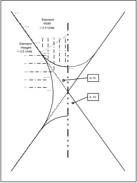
In the attached image, I have tried to show both the X-cusp and the Funny cusp models. In each case, I modeled the right side of the “square” coil to the left, and the bottom of the triangular coil above. For the Funny Cusp, the coils actually overlay one another and the corners meet at the point in the middle which is the vertex of the polyhedron. For the X-Cusp, the coils curve aside and leave a hole at the vertex.

Then, if I calculated the field from the modeled SIDE coil at the position of the star in the upper left quadrant in columns Q, R, & S, then I would also calculate the field at the position of the star in the lower right quadrant in columns Z, AA, & AB. This would be the same, but 180 degrees out of rotation as the field that would have been obtained at the position of the star in the upper left quadrant from the side of the OTHER square coil. Clear?

I will want to make these 4 wire segments explicit and independent before I can apply this model to the further problems that I have in mind.
I think that will be easy enough. Do you concur?

I suppose it wouldn't be too hard. You would just duplicate the Side and Top models from columns A,B,C... out to S and leave off the T thru AB. The superpositioning logic would also have to change, but that should be easy. Tedious, but not difficult.

I used arbitrary units of distance and amp-turns and did not include any constants. These values are all relative to an arbitrary unit.

That was what I was afraid of. I think I can turn the units into T by multiplying by 10e-7 (=mu0/4*pi) instead of by 100 at cells O52, Q52 & R52.
Are the length units real units? Or, do I need to convert them to meters of an actual machine to be modeled too?

The X-cusp model was sized to give a reasonable gap between the two square magnets assuming a set minor coil radius of 10 units. With that dimension, there are 6 units between the curved coil corners. Scale as you need. Please note that I do NOT have the curvature of the sphere in the model. It would be doable, but perhaps a pain.

I suppose I have to because none of the models we are considering for the near term are anywhere near 70 by 100 meters across the X cusp area.
That would change the loop paths columns A, B & C
and it would change the Table's X axis and Y axis numbers on the other worksheet (PlaneX) containing the large table.
I can then crank up the amps to get reasonable numbers.
Is that correct?
Did I get all the conversions?
Do I need to make the conversion somewhere else instead?

I think you can do the proper conversions in the constant rather than change all the model numbers. The basic equation is on the first sheet. Just do a dimensional analysis of the equation to determine the residual units and include a conversion factor.

Also on the "summary" sheet you have a "minor radius" that seems to go nowhere. Was that just a handle for future expansion?

No. It is used. The value is transferred to cell I2 in each of the calc sheets and then used to approximate the fall-off of the field inside the coil. It has no effect when looking at the field 10+ units away in the z direction, but smooths out the results for the z=0 case.

and, how did you generate the wire curves shown on "X-Xusp" columns A, B & C?

The center of the curvature is 70 units away from the line of symmetry sideways and 50 units vertically. This was used as a simplification. I used the same proportions to line up the straight runs of the coil. The real angle would be slightly different, by about a half degree. I then drew circular arcs between the points where the CL of the coil crossed the lines between the centers of curvature. There is a dotted line that shows that the upper portion of that line between the centers of curvature in the image below.

[tombo]

It seems to have gotten fuzzified during conversion to jpeg to photobucket to here.
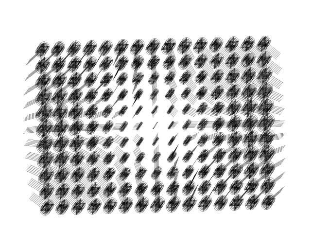
Again ball dia and line length are proportional to field strength and line direction is field direction.
The scale is Teslas with an adjustment to fill the view reasonably, and to make the lines longer than the balls so we can see them.

This is X-cusp configuration.
You can see the fields coming in to the center from top and bottom and leaving to the left and right.
The components into and out of the page are hard to see.
They are even hard to see looking in 3D CAD.
I've got to get the ergonomics better before tightening up on the resolution.
My biggest headache today was trying to keep excel stable. It does not seem to want to do things the same way twice.
If I can get an estimate of the electron velocity at this point I will do one giving the balls the gyro radius.

[KitemanSA]

Two questions.
At what Z level, mid plane or z=10?
Did you rotate it or just shorten it?

[tombo]

This is still just a random shot of work in progress
I'm not really happy with it yet, although it is getting almost useful.
The z axis is very foreshortened from this viewing angle.
That angle is to show all the field direction/strength lines between the balls. And besides at least one of the axes needed to be foreshortened.
Trying to show 6+ degrees of freedom on a 2D sheet of paper is unsatisfactory. (to put it mildly)

I rescaled it from your numbers to make them closer to the actual meters of a large scale machine.
So your 70 is now 0.70 for example.
(comments? clarifications? new list of actual size of the cross-connected wires?)

That said:
In the above picture
The X scale runs from +0.70 to -0.70 in steps of 0.10
The Y scale runs from -0.50 to +0.50 in steps of 0.10
The Z scale runs from -0.50 to 0.00 in steps of 0.10

Question for you:
The "minor radius" acts on an unlabeled column (4 ea) of the spreadsheet between "R" and "B field".
What do you mean by "minor radius" and what does that column do?
The scale change changed it from 1.00 to a quite different number so I can now no longer overlook it.

[KitemanSA]

Question for you:
The "minor radius" acts on an unlabeled column (4 ea) of the spreadsheet between "R" and "B field".
What do you mean by "minor radius" and what does that column do?
The scale change changed it from 1.00 to a quite different number so I can now no longer overlook it.

Think that this is a part of a torus (flattted on four sides into a rounded square) with a major radius that is quite large and a minor radius that is the number you put in that cell. It is the dimension of the cross section of the magnet coil. Slice the magnet ther and look end on and you have a bunch of wires coming at you in a bunch that many units across.

It is used in a kludgy form to modify the field when you calculate it very close to the magnet. Without it, the magnet is treated as an infinitely thin coil so the filed as r (standoff in this case) goes to zero becomes infinite. By inputting the minor radius, the current gets reduced by the ratio of your standoff from centerline within the coil divided by the minor radius, quantity squared. Clear?

thsi of course assumes that the current is evenly divided across the section and that B field generated by current outside the standoff gets canceled.

[tombo]

That is what I thought you were trying to get at, but I was not sure.

By inputting the minor radius, the current gets reduced by the ratio of your standoff from centerline within the coil divided by the minor radius, quantity squared. Clear?

No, not exactly clear yet.
The radius of the conductor or the radius of the casing?

Why would it deviate from Biot-Savart?
Where did you get your equation for the region close to the wire?
I would expect it to follow Biot-Savart right down to the casing where it falls straight to zero (for these purposes).
This avoids the singularity.

The analogy is gravity.
The gravitational acceleration looks and acts like the mass of the earth is concentrated at the center right down to the point where the tomato hits the street 4000 miles short of its target.

[KitemanSA]

The radius of the conductor or the radius of the casing?

In this case I have no case, just a schmear of conductor that approximates a bundle of individual wires. The schear is modeled as a centerline and acircular cross section (approximately).

Why would it deviate from Biot-Savart?

It doesn't really, but B-S gives you the field outside the wires, and it sums up all the idividual fields when you calculate a bundle of wires. Thus any field due to current outside the location cancels itself out. TaDaa.

Where did you get your equation for the region close to the wire?
I would expect it to follow Biot-Savart right down to the casing where it falls straight to zero (for these purposes).
This avoids the singularity.

I caused mine to fall to 0 based on the amount of current still inside the location. This avoids the edge singularity your way produces (if I understand your way).

The analogy is gravity.
The gravitational acceleration looks and acts like the mass of the earth is concentrated at the center right down to the point where the tomato hits the street 4000 miles short of its target.

But if you could dig a hole all the way to the center of the earth under the tomato, the tomato's acceleration would decrease with depth and be proportional to the amount of mass still inside the radius of the position of the tomato.

[tombo]

I caused mine to fall to 0 based on the amount of current still inside the location. This avoids the edge singularity your way produces (if I understand your way).

I don't really care about the field inside the conductor.
My only concern is the field in the plasma region.

The singularity is a real one at the conductive surface of the magrid.
Most of our real concerns are not very close to the magrid but out in the cusp region anyway.

Another nice feature about dropping it to zero at the surface is that the outline of the magrid should show up automatically as a hole in the displayed region of field.

The spreadsheet model could easily be changed to sum up the fields from say a dozen wires in a circle or a space filling 7 or 19 wires.
It could even subtract that result from the field generated by the same current in a single wire to give checksum=error signal that should be zero if the theory and implementation are correct.

It would also be good to double check the model against known configurations such as the field in the center of a circle or of a square turn.

Let me ask explicitly another question that I asked implicitly before.
Is 0.70 meters by 0.50 meters and the minor radius (thickness) of the magrid = 0.10 meter the real size of the cusp region in question?

[KitemanSA]

Another nice feature about dropping it to zero at the surface is that the outline of the magrid should show up automatically as a hole in the displayed region of field.

Won't show up real nice since I used the actual distance of the field point relative to the mid-point of the line segment, not the distance normal to the line segment. This works ok when schmearing, but may not when cutting things off. Depending on your discretization, the coil may look like a string of beads.

The spreadsheet model could easily be changed to sum up the fields from say a dozen wires in a circle or a space filling 7 or 19 wires.
It could even subtract that result from the field generated by the same current in a single wire to give checksum=error signal that should be zero if the theory and implementation are correct.
It would also be good to double check the model against known configurations such as the field in the center of a circle or of a square turn.

It runs slow now. But you have it, play with it.

Let me ask explicitly another question that I asked implicitly before.
Is 0.70 meters by 0.50 meters and the minor radius (thickness) of the magrid = 0.10 meter the real size of the cusp region in question?

For the full size unit, it seems a bit small. MSimon came out with a minimum dimension of about 29cm. And that was square without a case. I suspect a minor radius of at least .2m, maybe even .3m will be needed, but I haven't checked MSimon's work too carefully.

[tombo]

distance of the field point relative to the mid-point of the line segment, not the distance normal to the line segment.

good point

If the bead density is high enough it should show where it is well enough.
I may yet have to draw the coil wire explicitly from the wire path segment list. If so, so be it.

I have seen him present numbers from 8" dia on up.
Someday maybe I will run the heat flow numbers and come up with my own opinion. I think almost any amount work that gets the thickness down is well spent and has a large multiplier effect.
It may go down as a result of the majority of alphas exiting through the nodes & deflected away from the magrid itself. That effect is a welcome piece of design slack.

So the 70cm and 50 cm numbers for the rectangular opening are what you are working with?

[MSimon]

My latest understanding is that with pBj the heat loading is about zero (well close enough) due to the alphas exiting from the cusps. This should happen at fields above 1 T (at the center of the coils - i.e. in the center of the donut hole).

So only one layer of water may be needed (or maybe none). Eight inches is probably a good start and maybe six inches will do or even less.