Hmmm.
Obviously, this isn't as clear-cut as I thought. First, this simulation implements an analytic expression for the off-axis magnetic field of a thin current loop using elliptic functions. Each of the six loops is modeled as a set of loops to form the magrids, and the resulting fields (in the 2D plane of regard) are obtained by a linear superposition ("summing up") of the individual field vector components.
(Ref:
http://www.netdenizen.com/emagnet/offax ... ffaxis.htm for the expression for the off-axis field vectors)
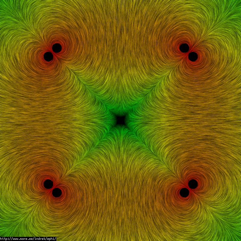
My first concern is to make sure that the analytic model for the thin loops is correct. Here is a test plot of a one-meter radius loop carrying one Ampere of current. The loop is centered at the X-axis, and current flows so that the B-field points in the x direction.
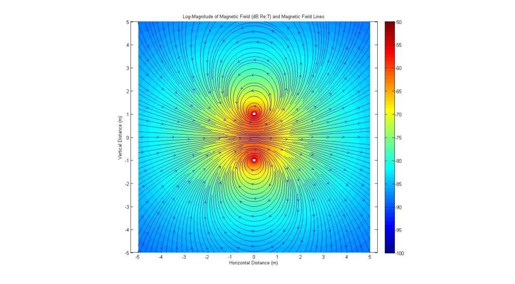
The streamlines look about right, so now I need to check that the magnitude is correct. For this, I compute the field strength on the x-axis, and use the well-known result for the on-axis field strength of a current loop. The plot is shown below.
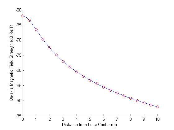
The blue line is the analytic result using the off-axis code, and the red circles are the results using the on-axis equation. The strength is shown in decibels re: one Tesla. It looks like the magnitude of the simulation code is about right, too.
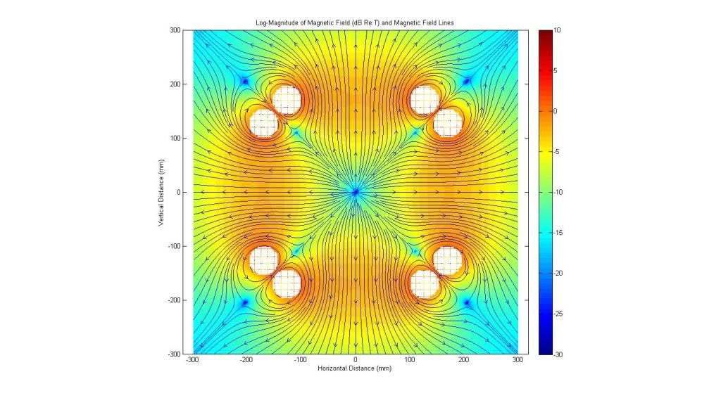
So, now the question is: does it make any sense that a "stagnation point" would show up in the model just inside of the "funny" cusp?
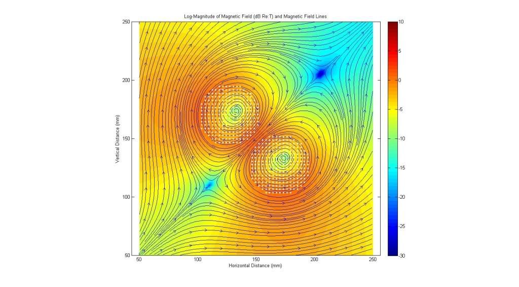
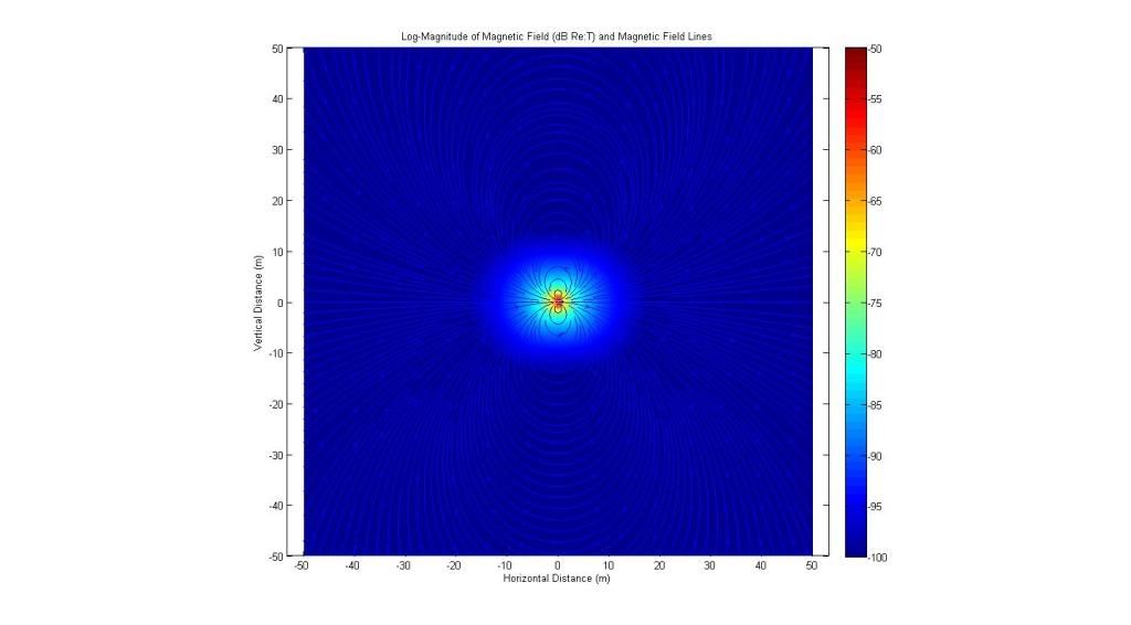
Here is an example of a null field using the same one-meter/one-ampere loop earlier. Here I have added a horizontal B-field that is exacly equal
and opposite to the loop field at +/- 2m.
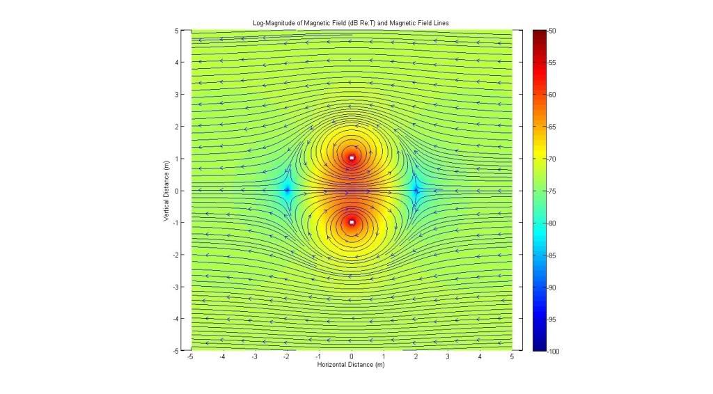
Note that the field goes to zero (as expected) at +/- 2m, and that the field forms something of a "bubble" around the loop. This happens because the horizontal field is stronger than the loop field at distances beyond 2m, but the loop field dominates at distances less than 2m. Nothing too unexpected if we think about the vector addition of the individual field components.
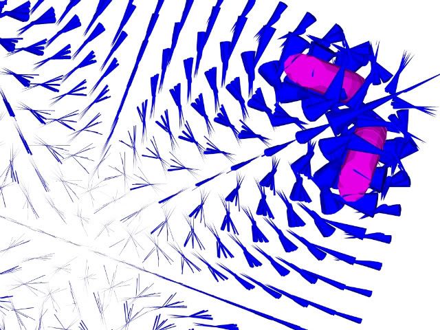
So what happens with the field components at the "stagnation point" just inside the upper-right-hand corner of the original plot? Here is a representation of the six individual B-field vectors:
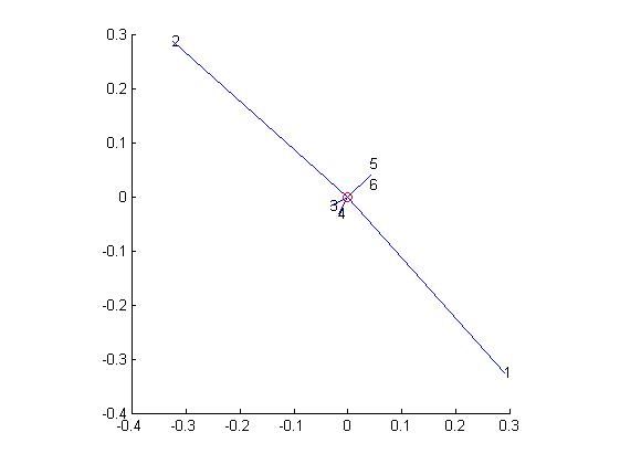
In the figure above, the blue lines represent the B-field vectors (linear magnitude and direction) for the six grids. The numbers at the end of each line indicate which grid produced which vector. "1" is the vertical grid on the right, "2" is the top horizontal grid, "3" is the vertical grid on the left, "4" is the bottom grid, and "5" and "6" are the out-of-plane grids above and below the 2D analysis plane. The red circle at the center represents the vector sum of those six components, and is indeed very close to zero. If you spend some time pondering this plot and thinking about how the field lines form around each individual loop, it seems to make sense that there could be a cancellation of the field at a point just inside the "funny" cusp.